Optical Triggering Results

Coil A

The following speed test results show that the optical triggering method compares favourably to the optimal open loop results. Table 1 shows the speed values for all projectile types.

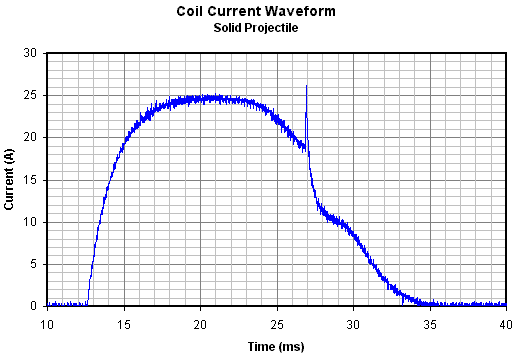
Table 1: Optical triggering speeds for all projectiles.

Notice that there are slight differences in the speed values obtained for members of each type of projectile. The reason for this is most likely due to variation in the dimensions of the individual projectiles although the effect could simply be statistical 'noise'.

Now let's look at the coil current trace. Fig 1 shows a typical waveform for solid projectile 1.

Fig 1. Optically triggered current waveform.

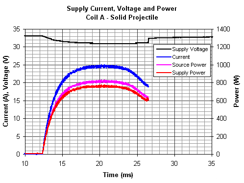
I've plotted the data in a spreadsheet programme so that additional detail can be shown. The time axis values may seem a bit odd but this is due to the sampling method used by the 'scope - it collects data continuously while waiting for the trigger threshold. It retains some of this pretrigger data so that any events occuring shortly before the trigger can be recorded.

The shape of the current waveform is essentially identical to that obtained in the open loop triggering. There is no reason for it to be different since the mosfet module is being driven by a signal of similar magnitude. One thing which is noteworthy is the sharp current spike at the end of the conduction phase. This represents the turn off point and it is actually present in all of the open loop current traces as well. The oscilloscope display doesn't usually show it because the screen display plots the trace by using a limited number of the actual data points that were recorded. I didn't mention it before because I was leaving this aspect of the investigation to the switching experiments.

We can look at the source power curves as shown in fig 2. I'm using the term 'supply power' to indicate the power delivered by the source to the coil and switching device - the product of the source terminal (supply) voltage and current. 'Source power' describes the total power generated inside the source - the product of the open circuit voltage and current. The difference between the source power and supply power is the power loss due to source internal resistance. The current and power curves stop at the turn off point because after this event the supply is disconnected from the coilgun.

Fig 2. Voltage, current, and power curves.

Notice that the maximum voltage drop across the source during this firing is quite small at around 2V. This is to be expected since the peak current drain is only about 25A. The power curves indicate that the maximum power loss in the source internal resistance is around 50W.

We can determine the overall system efficiency by calculating the total energy supplied by the source and comparing this to the resulting projectile energy. Table 2 shows the resulting efficiencies for a single commutating diode and a 10 segment series diode array.

Table 2. Efficiency comparisons for solid projectile.

I've made a distinction between the coilgun efficiency and the overall efficiency because when you read the specifications for an electrical machine such as a motor, the efficiency is just quoted as the machine efficiency. Efficiency ratings don't usually take into account the losses incurred in the source and transmission lines. I think it's important to make this distinction since overall coilgun system efficiencies are often incorrectly compared to the machine efficiencies of electric motors. That said, the overall system efficiency is perhaps the correct way to rate a coilgun since the energy source is an integral part of the design.

It's worth noting here that the values for both efficiency rating methods are quite close. The reason for this is simply that the low current demand leads to a small internal loss in the source. We will find that as the current demand increases there will be a proportionally larger gap between these efficiencies.