Optical Triggering Results

Coil B

Again we can compare the maximum muzzle speeds obtained open loop triggering and optical triggering. Table 1 shows the resulting speeds for each projectile type.

Table 1. Comparison of maximum open loop speed and optical speed.

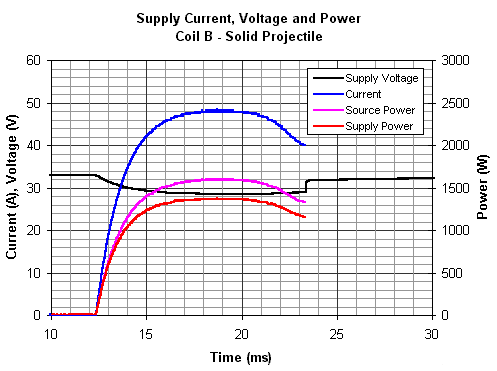
Now we can see that the optical method gives a slightly lower muzzle speed with this coil. The difference is small and indicates that the optical timing setup is close to ideal.

Looking at the operating curves in fig 1 shows that the difference between the supply power and the source power is increasing due to the greater current demand.

Fig 1. Voltage, current and power curves.

Table 2 contains details of the energy and efficiencies for a solid projectile.

Table 2. Efficiency comparisons for solid projectile.

We can see that all the efficiency ratings for coil B are somewhat better than those for coil A, also, the proportional difference in efficiencies has increased as expected.