|
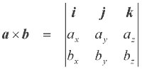
Mathematics 1,2 1. Vector Cross Product I'll use the standard i,j and k to denote the unit vectors along the x,y and z directions respectively. If we have two vectors, a and b, the vector product is given by
This can also be written as the determinant of a 3x3 matrix as follows
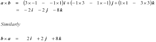
Examples: Vector a = i + 3j - k and vector b = 3i+ 1j - k. Find axb and bxa
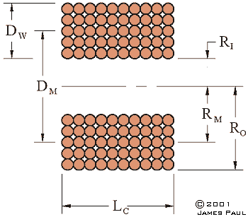
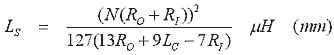
2. Inductance Equation This equation is presented in "Coil Design and Construction" by B.B. Banabi. It can be used to find the self inductance of an air cored solenoid coil. The range of dimensions over which this equation can be accurately used is unclear, the book makes no mention of its limitations. The equation is originally expressed with imperial units but it is straightforward to convert these to metric if desired. The coil parameters are illustrated in fig 2.1.
Fig 2.1
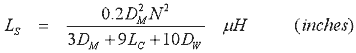
Note that DM and RM are the mean diameter and radius respectively. The self inductance equations are:
Eqn 2.2 uses radii instead of diameters although this doesn't need to be the case. You can configure the equation anyway you like so long as you apply the correct conversion factors. 3. Standard Resistance Equation This equation is used to calculate the resistance of a conductor based on its dimensions and resistivity.
Fig 3.1
where
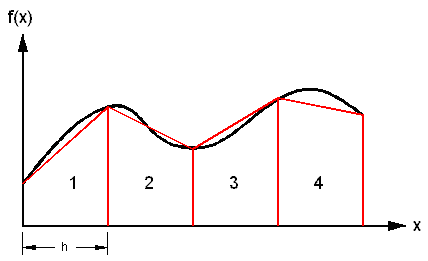
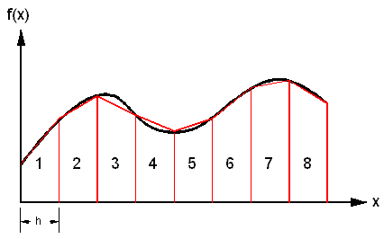
4. Numerical Integration - Trapezium Method This method of numerical integration uses the trapezium approximation to calculate the definite integral - the area bounded by the curve and the axis. I'm not going to go into details about how to develop the equation - the trapezuim rule. What is useful about this method is that it uses a range of x-values and y-values to determine the integral. Now often these values will be generated from some equation but when it comes to the integrating the DSO waveform we already have a range of time and voltage values which can be readily integrated using the trapezium method. In fact Matlab has a trapz(x,y) function which will calculate the integral based on the range of x and y values which are passed to it. Only a minimal amount of spreadsheet formatting is required to get the DSO data into a useable form. One thing to note is that the trapezium method only gives approximate results if the y-values are derived from a continuous function. The area of the trapezium will either overestimate or underestimate the true value by a some amount. The result becomes more accurate as the number of approximations increases (smaller h). The full DSO data spans 4096 points so the trapezium method should give a good approximation.
Fig 4.1 Trapezium approximations
Fig 4.2 Smaller h value gives a more accurate result
|