|
Induced Voltage Sensor Simulation
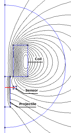
The building and testing of induced voltage sensors is a time consuming task so it makes sense to try out design concepts in virtual experiments where the investment in time and materials is much reduced. FEMM provides a means of accomplishing this virtual prototyping phase. The major simplification in this analysis is that the coil current is fixed. Firstly we need to construct a model of the coil, projectile and sensor, then run simulations with the projectile moved incrementally from the start to end positions. A LUA script is the best way to approach this as it automates the simulation and data extraction procedures. Fig 1 shows the model with the sensor coil located 9 mm from the rear of the drive coil (as is the case in the test coil). The projectile starts with its leading face flush with the rear face of the coil (ie delta = 0). The red line, which terminates at the mean radius of the sensor coil, indicates the integration path used to calculate the total flux passing through the sensor. The sensor doesn't actually contribute anything to the model since the integration line is given start and end coordinates explicitly in the LUA script, however it is included simply as a visual reference when working on the model geometry. The current density in the coil is set to 100 MA/m2 which is translated from a coil current of around 200-400 A, for typical coilgun wire diameters.
Fig 1. Model geometry showing initial projectile position and integration line (red).
The information we require is the voltage our sensor generates for a given coil current, projectile position, and velocity. The first step is to gather flux linkage data for the sensor coil. The flux linkage data is found through the B.n integral which returns the total flux passing through the integration line. We then take the flux linkage data and calculate the rate of change of flux linkage with displacement as shown in table 1. The voltage
from the sensor coil is dependant on the rate of change of flux
linkage with time so by multiplying d
Table 1. Voltage per turn with projectile velocity of 10 m/s
Fig 2. Induced voltage at various positions with projectile velocity of 10 m/s
Last Modified: 12 Feb 2004 |
|

 /dx
by dx/dt (the projectile velocity) we get the voltage per turn developed
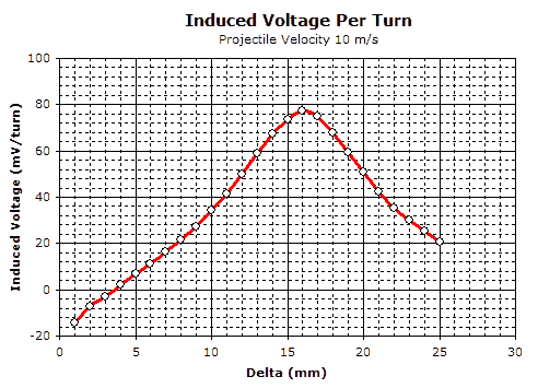
in the sensor. A velocity of 10 m/s is used as an example. Graphing
this we get the curve shown in fig 2. The peak of this curve occurs
at a delta of 16 mm (4 mm before the standard optical trigger goes
LOW) and has a value of just under 80 mV/turn, so the number of
turns required to get a useful voltage is of the order of 100. The
sensor coil in the final test coil design has approximately 150
turns.
/dx
by dx/dt (the projectile velocity) we get the voltage per turn developed
in the sensor. A velocity of 10 m/s is used as an example. Graphing
this we get the curve shown in fig 2. The peak of this curve occurs
at a delta of 16 mm (4 mm before the standard optical trigger goes
LOW) and has a value of just under 80 mV/turn, so the number of
turns required to get a useful voltage is of the order of 100. The
sensor coil in the final test coil design has approximately 150
turns.