|
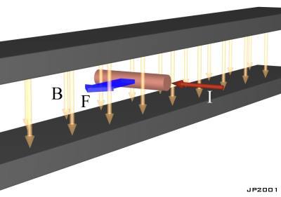
Electromagnetic Basics 14. Electromechanical Energy Conversion - The core principles of electromechanical energy conversion apply to all electrical machines and the coilgun is no exception. Before we consider the coilgun let's imagine a simple linear electric 'motor' consisting of a stator field and an armature immersed in the field. This is illustrated in fig 14.1. Note that in this simplified analysis the voltage source and armature circuit have no inductance associated with them. This means that the only induced voltage in the system is due to the motion of the armature wrt to the magnetic induction.
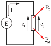
Fig 14.1. Primitive linear motor. When a voltage is applied across the ends of the armature a current will be developed according to its resistance. This current will experience a force (I x B) causing the armature to accelerate. Now from the earlier section on electromagnetic basics we illustrated the fact that a voltage is induced across a conductor moving through a magnetic induction. This induced voltage acts in opposition to the applied voltage (Lenz's Law). Fig 14.2 shows the equivalent circuit in which electrical power is converted into thermal power, PT, and mechanical power, PM.
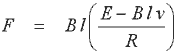
Fig 14.2. Motor equivalent circuit. Now we need to look at how the mechanical power developed by the armature relates to the electrical power supplied to it. Since the armature is positioned at right angles to the field induction, the force is given by a simplified version of eqn 11.4
so the instantaneous mechanical power is the product of the force and velocity -
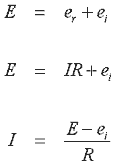
where v is the velocity of the armature. If we apply Kirchhoff's voltage law around the circuit we get the following expression for the current, I.
Now the induced voltage can be expressed as a function of the armature velocity
Substituting eqn 14.4 into 14.3 yields
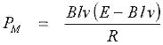
and substituting eqn 14.5 into 14.2 gives
Now let's look at the thermal power developed in the armature. This is given by eqn 14.7
And finally we can express the power supplied to the armature as
Notice also that the mechanical power (eqn 14.2) is equivalent to the current, I, multiplied by the induced voltage (eqn 14.4). We can plot these curves to show how the power supplied to the armature is distributed over a range of speeds. In order for this analysis to have some bearing on coilguns we'll give our variables values that are in keeping with the coilgun pistol accelerator conditions. Our starting point is the current density in the wire, from which we will determine values for the rest of the parameters. The maximum current density during the coil testing was 90A/mm2 so if we fix the wire length and diameter as -
then the wire resistance and current become -
Now that we have values for resistance and current, we can specify the voltage needed to drive the current -
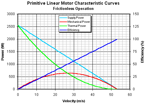
These are all the parameters required to plot the steady-state characteristics of the motor.
Fig 14.3 Characteristic curves for a frictionless motor model.
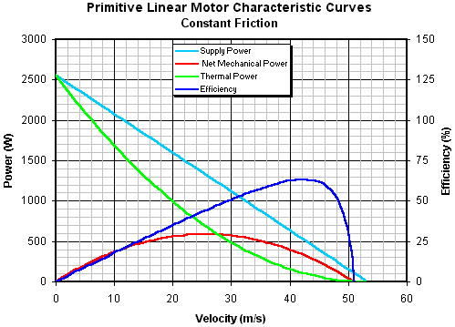
We can make this model a bit more realistic by adding a constant friction force, of say, 2 N, such that the mechanical power loss is proportional to the armature velocity. This friction value is deliberately large to show its effects more clearly. The new set of curves are shown in fig 14.4.
Fig 14.4. Characteristic curves with constant friction.
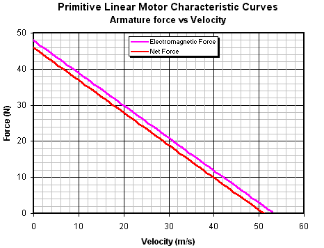
The presence of friction slightly modifies the power curves such that the maximum armature speed is slightly less the zero friction case. The most striking difference is the change in the efficiency curve which now peaks and then rapidly drops off as the armature approaches its 'no-load' speed. This form of efficiency curve is typical of permanent magnet dc motors. It's also worth looking at how the force, and hence acceleration, varies with speed. If we substitute eqn 14.5 into eqn 14.1 we get an expression for F in terms of v.
Plotting this expression we get the following graph -
Fig 14.5. Armature force vs velocity
Clearly the armature starts off with a maximum acceleration force that begins to decrease as soon as the armature starts moving. Although these characteristics give a snapshot of the various operational parameters at any particular speed, it would be useful to see how the motor behaves in time, i.e., dynamically.
|